The previous post mentions three basis vectors and a “dataset mean.” Here I explain how to find a good basis and what “good” means in this context.

The idea is to find a basis so that any spectral reflectivity can be expressed in the form: $$\mathbf s = \sum_i w_i\mathbf b_i + \mathbf b_\mu$$ where $i$ runs over all dimensions of the space (36 using Otsu et al.'s spectral data) and $\mathbf b_\mu$ is a constant term you can ignore for now. This is a very common problem and there are many general solutions. By far the most common one is the discrete Fourier transform, which turns arbitrary signals into weighted sums of sines and cosines.

Unfortunately, recalling that the goal is to upsample a color triplet (e.g. XYZ tristimulus values or RGB data), there are only three degrees of freedom to work with and so at most three weights can be determined. Reformulating the problem, $$\mathbf s = w_1\mathbf b_1 + w_2\mathbf b_2 + w_3\mathbf b_3 + \pmb\epsilon + \mathbf b_\mu$$ where all but three terms are lumped together into an error term $\pmb\epsilon$. I think it's clear that three sines or cosines (and a constant term) added together won't accurately reconstruct most spectra. There are far better purely mathematical models, such as Jakob and Hanika (2019).

Otsu et al. came up with a data-driven solution. Given enough measured data, you can use statistics and linear algebra to create a small basis that carries as much information from the original dataset as possible. The authors used principal component analysis (PCA) and a set of $N = 1{,}279$ measured reflectances.

Spectral reflectances are treated as random vectors, with each component a random variable. This method requires that their sample means are zero, so the measured data has to be adjusted first. Let $$\mathbf b_\mu = \frac{1}{N}\sum_i \mathbf s_i$$ which I called the “'dataset mean” in the previous article, then simply subtract it from measured spectra: $$\mathbf s'_i = \mathbf s - \mathbf b_\mu$$ From these the so-called data matrix, in this case an N x 36 matrix, can be constructed: $$X = \begin{bmatrix} \mathbf s'_1 & \mathbf s'_2 & \hdots & \mathbf s_{N} \end{bmatrix}^T$$ Now the idea is to use this to derive a basis that maximizes its variance or “significance.” I'll skip the proofs, as I'm not particularly well-versed in statistics and it would take me too much effort. The result is given by the eigensystem of the covariance matrix $\Sigma$ of $X$. The eigenvector of $\Sigma$ with the largest eigenvalue is the vector maximizing variance. The eigenvector with the second largest eigenvalue is perpendicular and has the second largest variance, and so on.

Let's take a look at the code. Assume that the measured data, sds, is an N x 36 array.

basis_mean = np.mean(sds, axis=0)
data_matrix = sds - basis_mean

A covariance matrix can be easily computed with np.cov, but a trick can be used. Because the column-wise means are zero, $X^TX$ is going to be equal to it up to a constant. The constant and any normalization can be ignored, as only eigenvectors are sought after.

covariance_matrix = np.dot(data_matrix.T, data_matrix)

The last step is the eigendecomposition. NumPy comes with a few algorithms, so it's not a problem. Because cov is Hermitian (it's a real, symmetric matrix), one can use:

eigenvalues, eigenvectors = np.linalg.eigh(covariance_matrix)

The bonus feature of eigh (aside from being more efficient) is that the eigenvalues are sorted in ascending order. The result is simply the last three columns of eigenvectors: the three basis vectors with the greatest variance.

Because zero-mean spectra were used to create the basis, it best describes primed spectra: $$\mathbf s' = w_1\mathbf b_1 + w_2\mathbf b_2 + w_3\mathbf b_3$$ Adding $\mathbf b_\mu$ to both sides, $$\mathbf s = w_1\mathbf b_1 + w_2\mathbf b_2 + w_3\mathbf b_3 + \mathbf b_\mu$$ recovers the equation from the beginning of this post and explains why the fourth basis vector has kept appearing. Notice that the error term is missing: the reconstructed spectrum is slightly different. I'll discuss this in part 3.

Thanks to Sıddık Açil for his his article on performing PCA in NumPy and Hao Xie for letting me know about it.

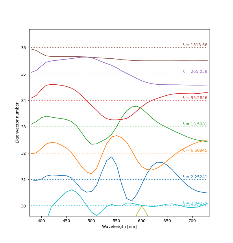
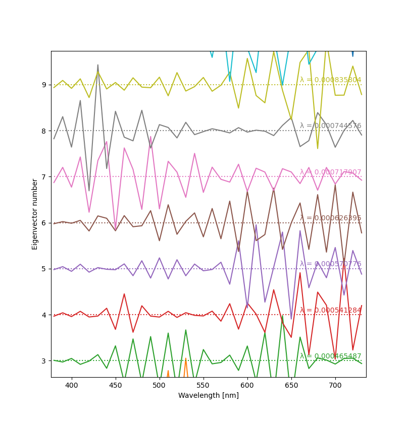
Below you can see plots of a few eigenvectors derived from Otsu et al.'s dataset. Since the vectors are meaningful only up to a constant, the Y scale can be chosen arbitrarily (and differently for each vector). The usual way to visualize them is to make a “ladder” plot, with the vectors stacked vertically according to their number. Eigenvalues are written on the right. The script is available here.

The results look oddly familiar. Notice that every next eigenvector (starting from the top) has exactly one more zero crossing than the previous one. My guess is that this has to be the case for them to be perpendicular and linearly independent. The eigenvalues are interesting too. They decrease very rapidly, with the largest few being much, much larger than the others. This explains why just three basis functions are enough for a good reconstruction.

As expected, the eigenvectors corresponding to small eigenvalues are noisy and random-looking.