Otsu et al. (2018), part 3

In the previous post I explained how PCA can be used to create a convenient basis for representing real-world reflectivities. The procedure uses a set of measured spectra to compute an orthonormal basis, sorted by variance or “statistical significance.” All but the three most significant vectors are then truncated. I called the difference between the actual spectrum and the reconstructed spectrum the error term .

Naturally the smaller the error, the better. Because is a vector, the authors chose the Euclidean norm (2-norm or L2) to represent the (scalar) error:

To get an idea of how well the method works in the general case, the authors would sum up reconstruction errors of all spectra in the dataset. I call this the total error :

where denotes the reconstruction error of , the -th measured spectrum.

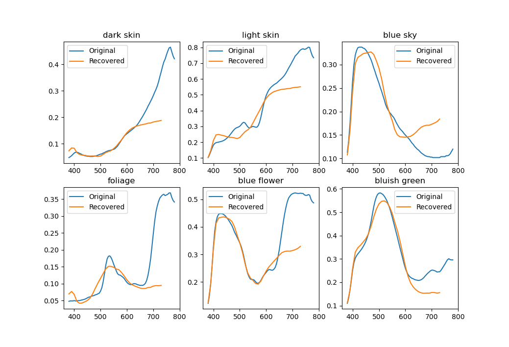
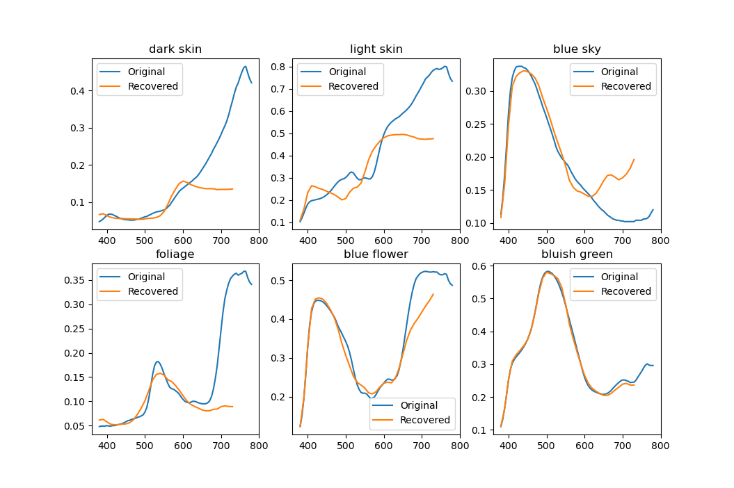
Using just one basis for everything isn’t ideal. The picture below shows reconstructions of a few colorchecker spectra. While by definition XYZ tristimulus values (and perceived colors) match perfectly, the spectra aren’t that close.

1. Clustering

The authors [1] decided to subdivide the CIE 1931 xy space using a binary space partitioning tree. Every node that isn’t a leaf divides its subspace in two with a horizontal or vertical line. Leaves, called clusters in the article, contain spectra that lie in their subspace. PCA is done for every cluster separately, creating a set of bases.

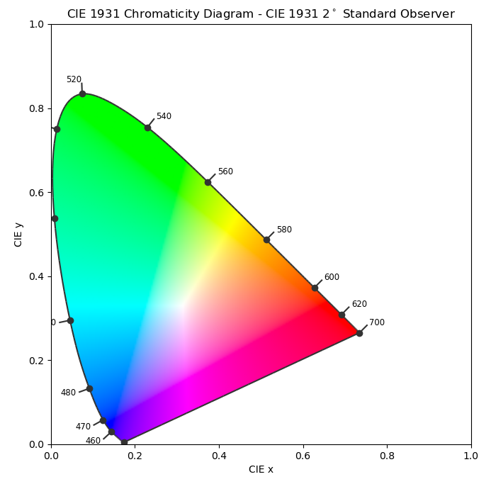
A quick note about CIE 1931 xy chromaticity coordinates. They’re derived from CIE 1931 XYZ tristimulus values:

They’re often used where only the chromaticity matters and not the lightness . When plotted, they give rise to the familiar “color triangle” or “horseshoe” diagram, pictured on the right.

The algorithm for creating an optimized clustering is described as follows.

• Search every possible new partitioning in the tree. For every color of every leaf, try partitions with a horizontal and a vertical line going through the color, assigning the color itself to the “lesser” part (to the left or below the line).
• Discard partitions that would create very small nodes. More on this later.
• Compute how each partition would affect the total error of the entire tree (the sum of of every leaf). Discard those that would increase it.
• Realize the partition that decreases the error the most.
• Repeat the entire process.

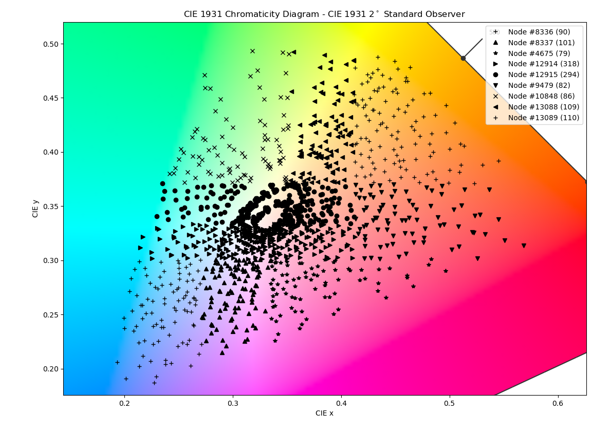
The algorithm terminates when no more partitions are possible or there are enough clusters. Authors chose 8 clusters, because of diminishing returns and dataset size concerns. You can look at the original implementation or my code. The article also has many more plots and comparisons than I post here, so it’s definitely worth looking at too.

Below are the results of running my code. I used the entire dataset of 1,279 spectra and optimized for 8 clusters. This takes about 3 hours on my dated i7 3770.

2. Minimum node size

I mentioned that nodes cannot be allowed to be split too finely. First of all, there have to be at least three spectra in a node for PCA to even work. Fewer will result in a singular and the algorithm simply won’t be able to continue. In practice, having few spectra is no good either. Below is a result of PCA decomposition done with just three spectra.

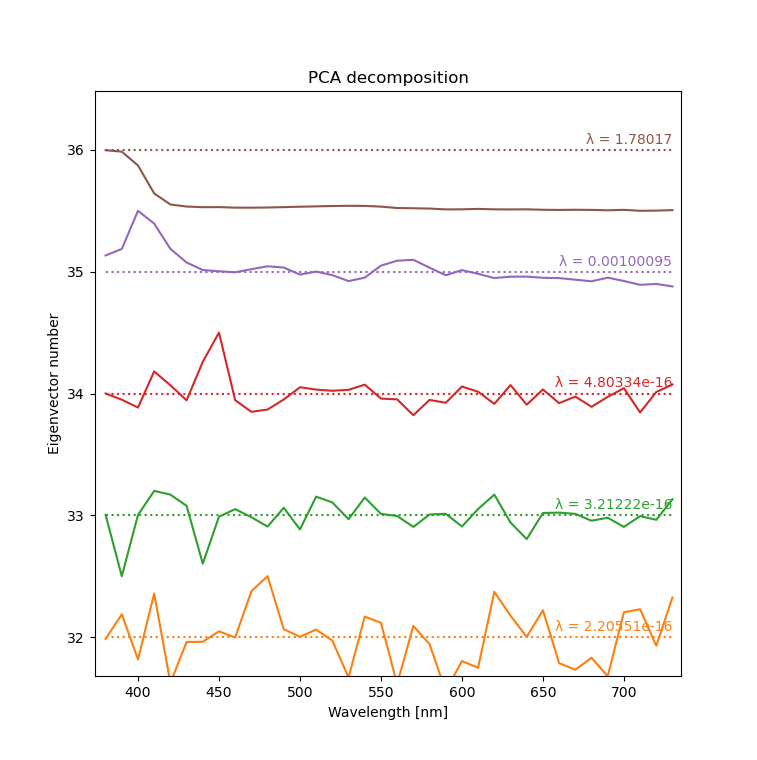
Only two eigenvectors are meaningful and the rest are basically noise. Trying to use this for reconstruction will create completely random-looking spectra, usually going way outside the [0, 1] range. Clearly a lot more data needs to be used to get useful results. In my program I (arbitrarily) set the minimum cluster size to the average cluster size divided by two and it seems to work pretty well.

But can reconstructed spectra exceed the allowed [0, 1] range even if the basis is good? Unfortunately yes, and this will be the topic of the next (and the last) post in this series.

Bibliography

- [1] H. Otsu, M. Yamamoto, and T. Hachisuka, “Reproducing Spectral Reflectances From Tristimulus Colours,” Computer Graphics Forum, vol. 37, no. 6, pp. 370–381, 2018, doi: 10.1111/cgf.13332.